Template for maps in R

data visualization with R

How to make a template for global maps.

# Packages needed
{
  library("ggplot2") # plotting
  library("sf") # spatial library
  library("rnaturalearth") # shape files for countries and coastlines
  library("rnaturalearthdata") # shape files for countries and coastlines
}

Shapefiles for countries and coastlines are available with the libraries rnaturalearth and rnaturalearthdata.

# Load data
world <- ne_coastline(scale = "medium", returnclass = "sf")
world_countries <- ne_countries(scale = "medium", returnclass = "sf")

Since we have a sf object, we can directly plot it:

ggplot(world) +
  geom_sf()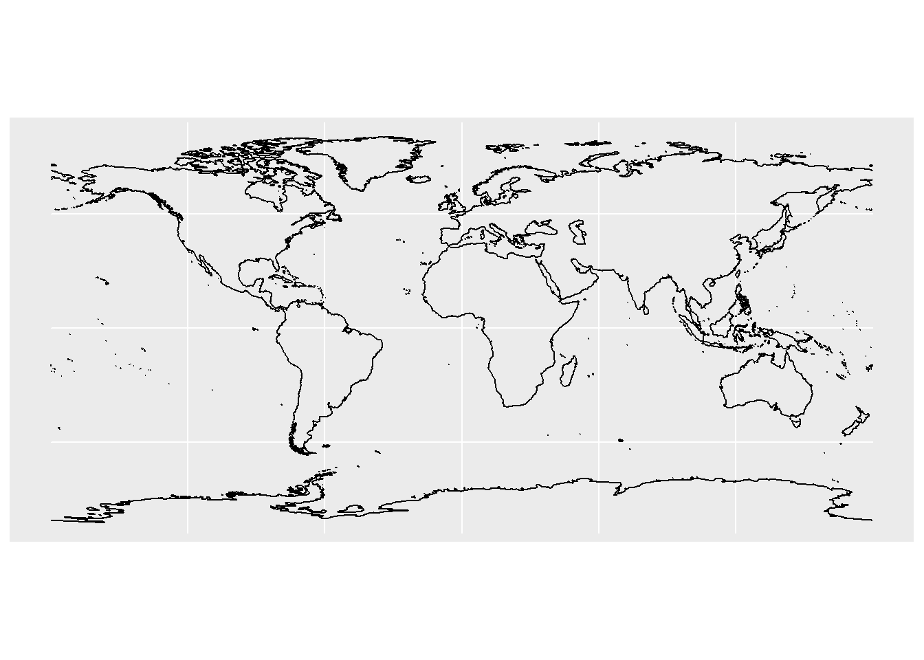

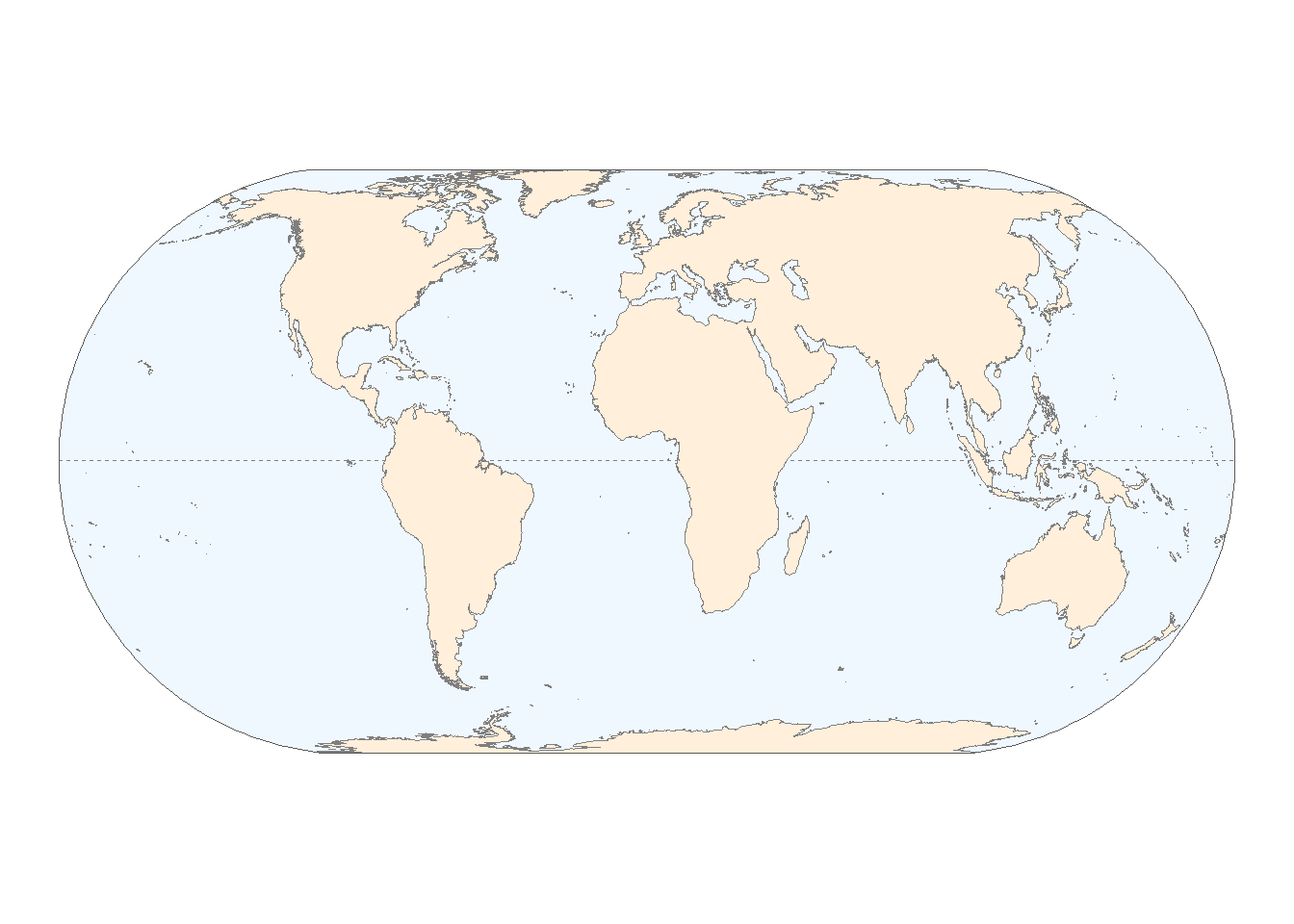
In the next steps, we: - add the Equator line
- Project the shapes with an equal-area projection
- Draw a background box, for the oceans and seas
- Combine everything into one plot

# Fixing polygons crossing dateline
world <- st_wrap_dateline(world)
world_countries <- st_wrap_dateline(world_countries)

# Eckert IV projection
eckertIV <-
  "+proj=eck4 +lon_0=0 +x_0=0 +y_0=0 +ellps=WGS84 +datum=WGS84 +units=m +no_defs"

# Background box
xmin <- st_bbox(world)[["xmin"]]; xmax <- st_bbox(world)[["xmax"]]
ymin <- st_bbox(world)[["ymin"]]; ymax <- st_bbox(world)[["ymax"]]
bb <- sf::st_union(sf::st_make_grid(st_bbox(c(xmin = xmin,
                                              xmax = xmax,
                                              ymax = ymax,
                                              ymin = ymin),
                                            crs = st_crs(4326)),
                                    n = 100))

# Equator line
equator <- st_linestring(matrix(c(-180, 0, 180, 0), ncol = 2, byrow = TRUE))
equator <- st_sfc(equator, crs = st_crs(world))

# Plot
plot_basis <- ggplot(world) +
  geom_sf(data = bb, fill = "aliceblue") +
  geom_sf(data = equator, color = "gray50", linetype = "dashed",
          linewidth = 0.1) +
  geom_sf(data = world_countries, fill = "antiquewhite1", color = NA) +
  geom_sf(color = "gray50", linewidth = 0.1) +
  geom_sf(data = bb, fill = NA) +
  coord_sf(crs = eckertIV) +
  theme_void()

plot_basis